Google Sheets Tutorial – How to Use Regex and VLOOKUP to Display Images from Google Drive

Images make many things better. And Google Sheets is one of those things.
The easiest way to add an image to Google Sheets is to simply insert one into your sheet.
But if you have added many images this way, you'll quickly tire of the multiple clicks it takes to do so. Especially if you have to add images often, or if you have to add the same images to multiple sheets.
In this article, you'll learn how to add many images from their URLs that you can dynamically toggle between in a dropdown list. We'll cover:
- Data Validation for creating a dropdown list
- Named Ranges to make formula references easier and cleaner
- The VLOOKUP function to display the right image from the dropdown list
- The REGEXEXTRACT function to extract a string from a URL (don't worry, it'll make sense 😉)
- The IMAGE function to display the image from a URL address
- We'll use the ampersand (&) operator as well as regular expressions (Regex)
- We'll also make our sheet look good by removing gridlines, changing the font, adding borders, colors, and a drop shadow effect behind tables
How to Setup the Project 📐
You can follow along with the sheet I'm using for everything we'll discuss:
https://docs.google.com/spreadsheets/d/1rFU2gPy6rU8IKFDmsxKHYCf0KGVHkcumQ5O5QCf156M/edit?usp=sharing
Make a copy if you want to edit it yourself.
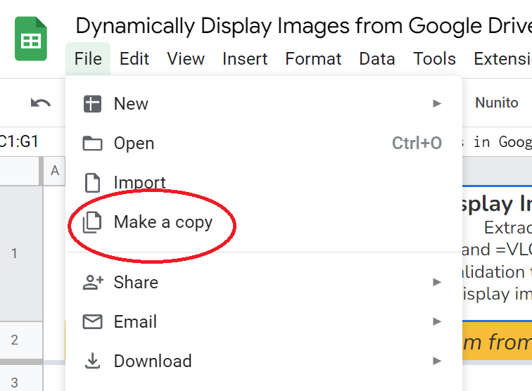
All cell and range references below will be from this sheet so you can easily look and see what I'm talking about.
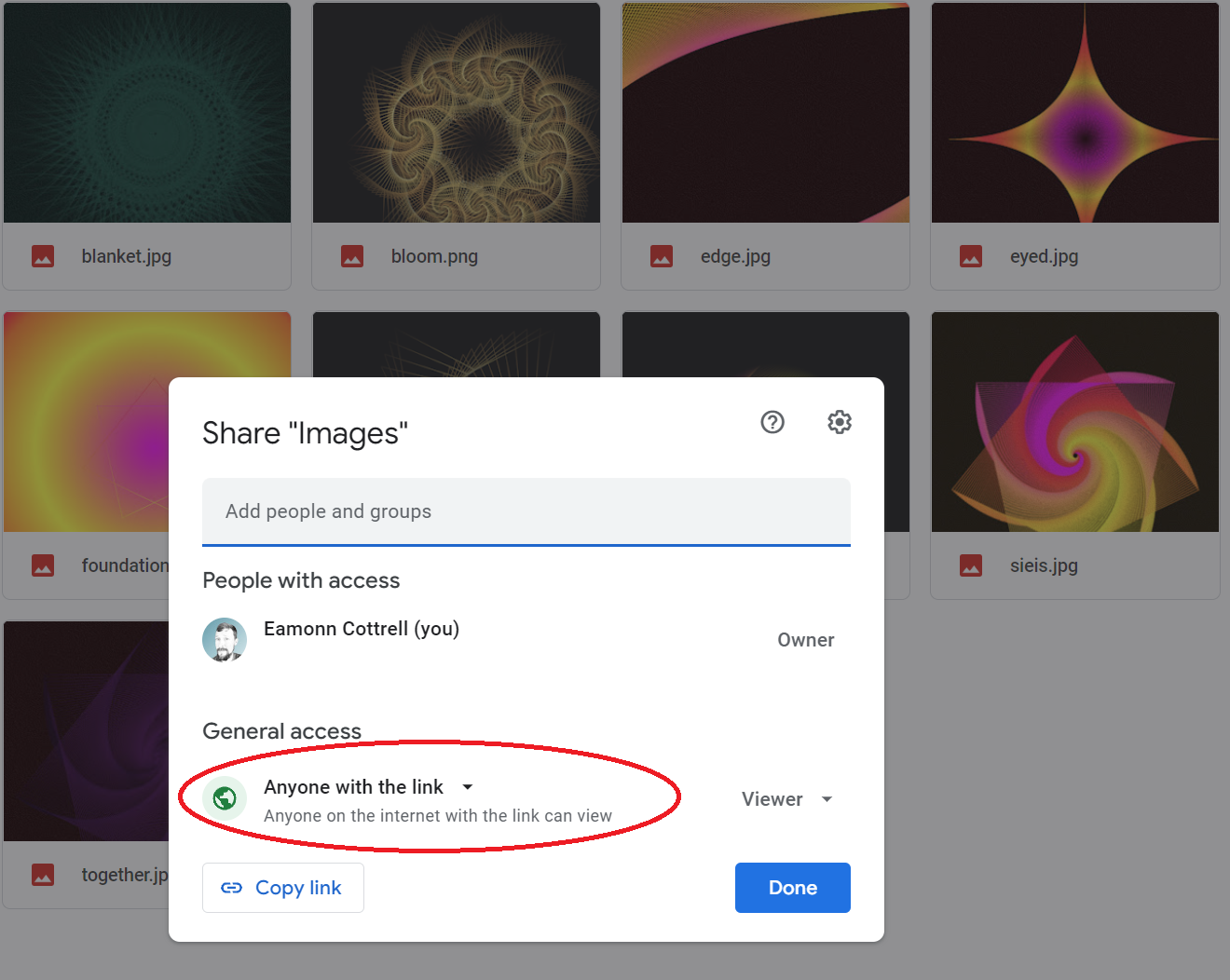
I've also made a folder of images here that is publicly shared so all this works. You don't have to make a copy of this unless you just want to 😀.
How to Use Named Ranges in Google Sheets 📛
Named ranges make life easier.
You don't have to use them, but it makes references in functions easier since you'll be writing the name of something instead of a sterile cell reference.
We'll use three of them:
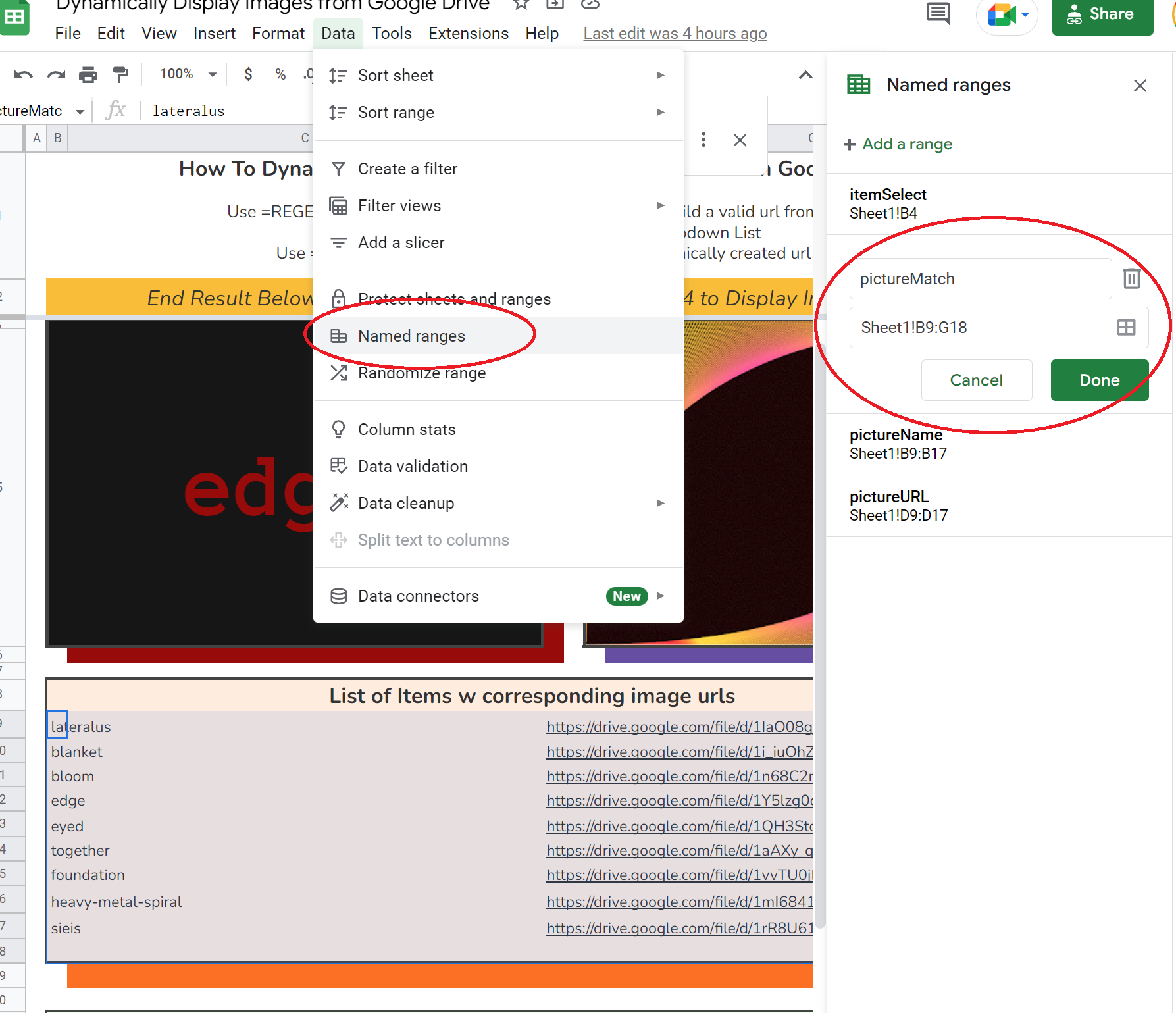
B4=itemSelectThis is the cell where our dropdown list will live.B8:G13=pictureMatchThis is the range for our VLOOKUP function. It contains the names of the pictures we'll display followed by their respective URLs.B8:B16=pictureNameThis is the first column of the pictureMatch range for referencing just the names in our data validation cell.
To create a named range, simply highlight the range, select Data -> Named ranges from the toolbar, and name it.
How to Perform Data Validation 📃
We'll use data validation to create a dropdown list in B4. Same deal here – just highlight the cell (or range) and select Data -> Data validation from the toolbar:
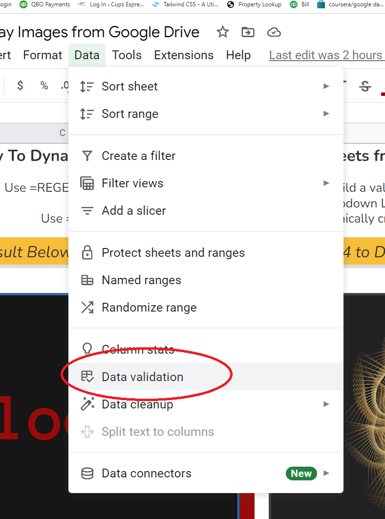
Select List from a range, and then =pictureName (because we named that range) for the range. Alternatively, you can declare the range explicitly.
There are additional options to configure if you want to change anything:
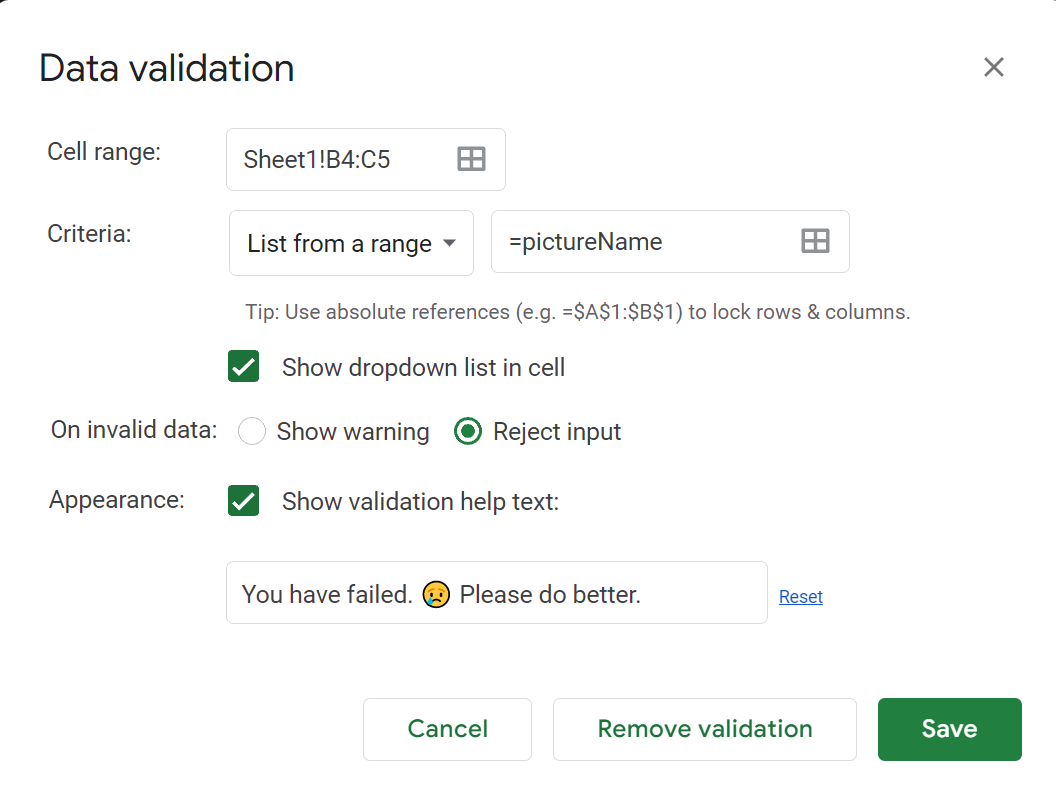
If you select reject input, you can have a custom message pop up whenever an invalid choice is entered:
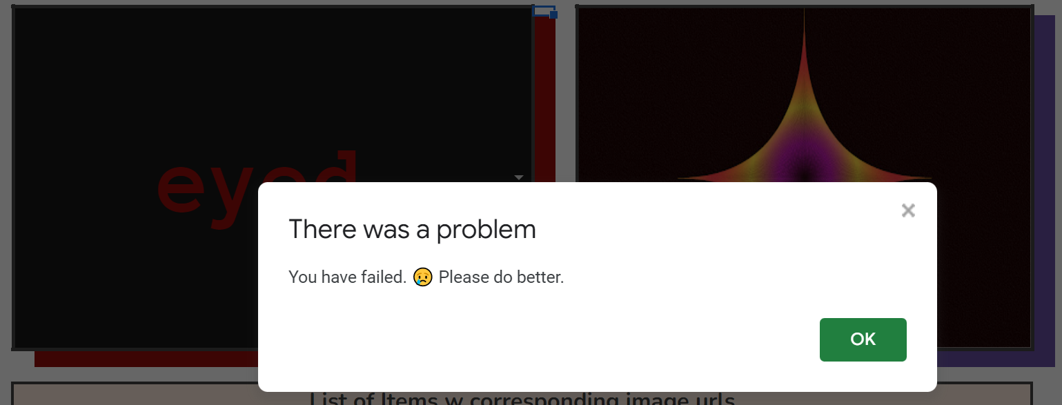
You might want to make your message more helpful than this one.
How to Use VLOOKUP 📊
VLOOKUP is an incredibly useful function. It takes four arguments:
=VLOOKUP(search_key, range, index, [is_sorted])

=VLOOKUP(itemSelect,pictureMatch,3,0)
We'll use itemSelect for our search_key and pictureMatch for the range because we want to find itemSelect in that range. Then the 3 for index gets the value in the third column in that range.
(It's 3 in our example because we merged the cells in columns B & C for our formatting, but VLOOKUP still counts both of them).
Finally, the zero sets is_sorted to FALSE. Our data is not sorted, and we want an exact match.
How to Use REGEXEXTRACT 💾
It happened: I found a real world use for Regular Expressions. 😳
This section of freeCodeCamp's Javascript certification was particularly confusing for me, and it was good to revisit a small portion of it here in the wild.
Because Google Drive is quirky, and we're sort of hacking a free option here, we need to alter the URLs to our images in order for the IMAGE function to work properly.
This Stack Overflow answer was helpful for me.
We need to build a URL by taking this:
https://drive.google.com/uc?export=download&id=###
and replacing the ### part at the end with the ID we extract with the REGEXEXTRACT function.
Looking at the URLs we copied over, we can see a pattern. Everything after the /d/ and then before the next / is the ID.
Here's an example of one of our image URLs: https://drive.google.com/file/d/1IaO08gj3GWIUQDAnzKEob62Gcl87ufuN/view?usp=sharing
You can see this at work by itself in B26 of the example spreadsheet as the function grabs everything between those two markers:
=REGEXEXTRACT(D9,".*/d/(.*)/")


This extracts everything between the /d/ and the /
How to Use the IMAGE Function 📷
Okay. We've got the disparate pieces figured out. I know the pieces fit. 🎵
Let's put them together.
All of our work was to get one cell ( B4 ) to provide data to the IMAGE function.
Image takes one argument and three other optional ones:
IMAGE(url, [mode], [height], [width])
We build the URL by combining the required beginning of the URL which I've got in J17 using the ampersand (&) operator with our REGEXEXTRACT function. And within our REGEXEXTRACT function we use our VLOOKUP function to get the URL of whatever image we've selected in the itemSelect cell.
Whew.
But, cool, right!?
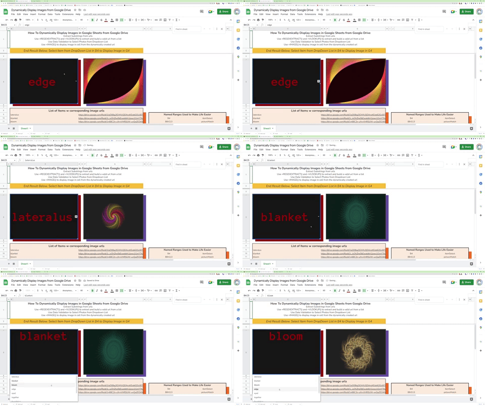
If you feel lost in a recursive nightmare, I encourage you to pull up the example spreadsheet and examine the parts of the function in F4 piece by piece. 👍
How to Format Your Sheet FTW 💯
These few details can turn up the volume 📣 on an otherwise mundane spreadsheet.

This is likely the only place you'll find a NIN gif in an article about spreadsheets today.
I love a hard drop shadow, and we can achieve this by manipulating the row and column sizes around a particular cell or range, using the merge cell option for our main range, and then using a fill color around the right side and bottom.
Click the lines between the column headers to drag and adjust the widths and heights of the columns and rows.
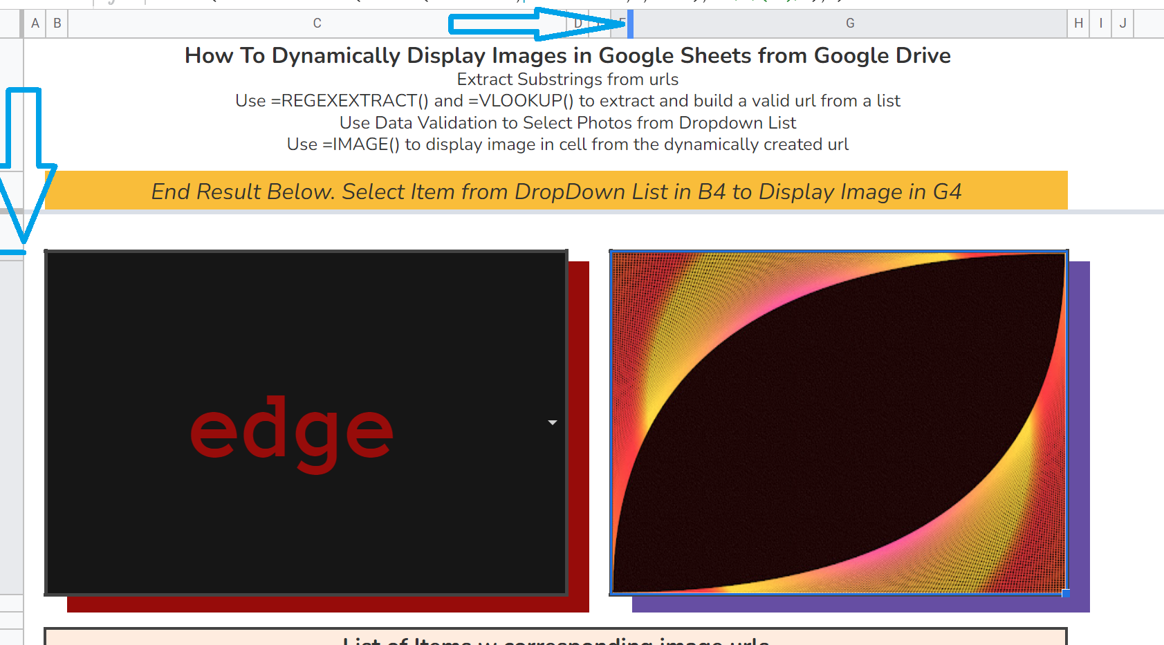
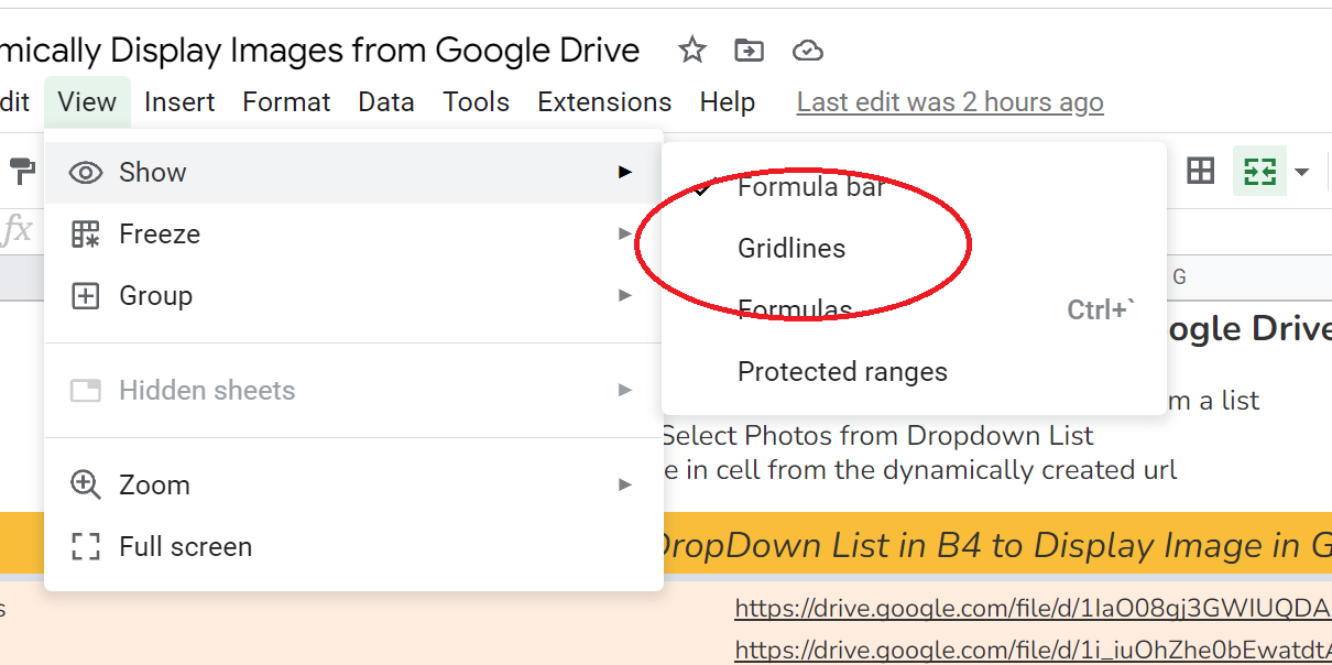
Cells are the main appeal of spreadsheets, but in some cases hiding the gridlines can make your sheet standout. I opted for this approach in this project.
Select View->Show->Gridlines.
As much as I appreciate Arial, I will typically opt out of the default font immediately.
Click the Font Dropdown in the Toolbar. It's usually smack dab in the middle:
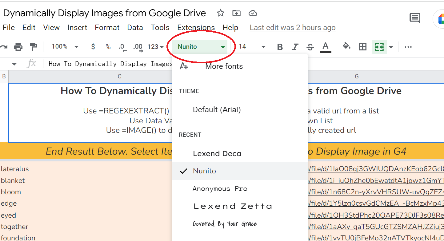
And just choose whatever font you'd like.
There you have it!
Thanks for Reading! 🙏
Follow me on Twitter to see more content like this: https://twitter.com/EamonnCottrell
Thanks!

About the author
- I'm an AI automations and strategy educator on YouTube. I also review products. I love ultrarunning. I'm the father of 4 kiddos.
Comments
Join the discussionNo comments yet. Be the first to comment.